Dynamic Mode Decomposition

January 21 2024

An overview of the Dynamic Mode Decomposition.

In college I got to do research on the dynamic mode decomposition. It’s an algorithm to break apart (decompose) a times-series matrix into exponentially growing or decaying (dynamic) parts oscillating at fixed frequencies (modes).

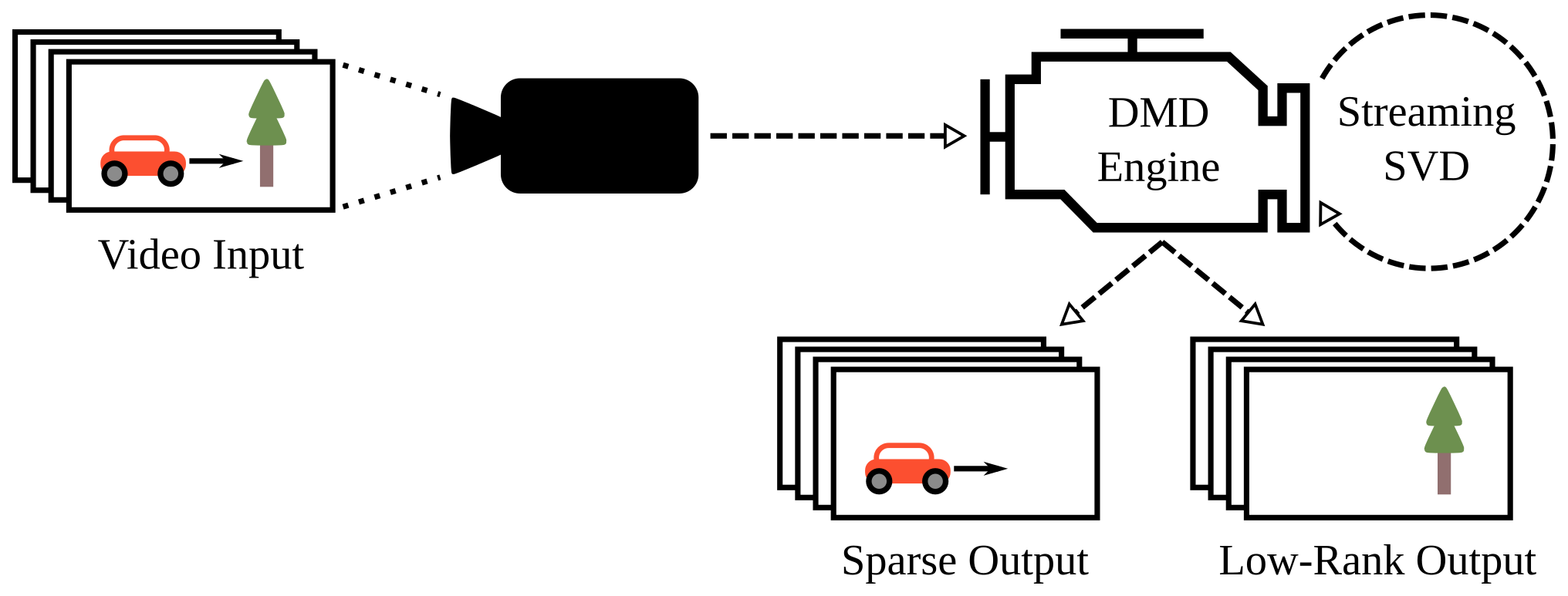
This is useful in analyzing changing motion, for example in fluid flows. It also can be used to remove the background from a video, by separating the high-growth or decay foreground from the relatively constant background. I’m intending this post to be a simplified, programmer-first explanation of why the DMD is interesting rather than a reference for the math or theory. I apologize in advance if I’ve messed up any of the equations or details, but I’ve done my best to check for their accuracy. Kutz et al.’s book Dynamic Mode Decomposition is a much better place to go for a formal explanation of the DMD.

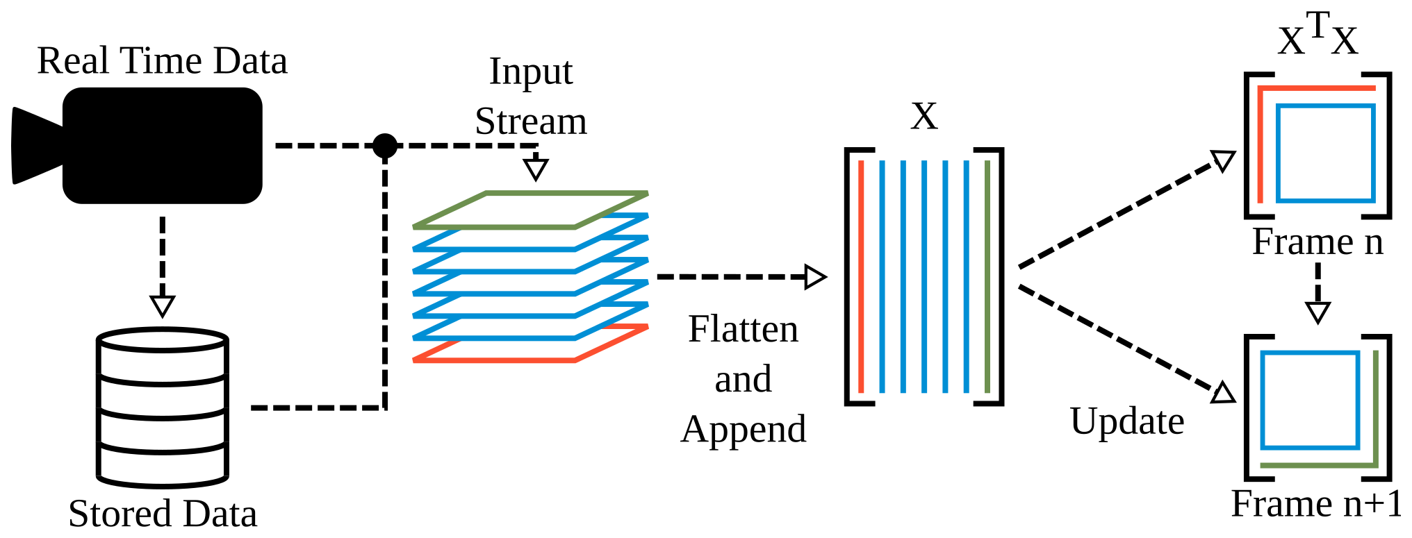
My small contribution to the DMD was making the GPU-accelerated implementation of the Streaming DMD, which lives on GitHub.

The source code to the figures on this page is available here. I recommend PyDMD if you’d like to play around with the DMD.

Overview

Rather than diving into the details of how you calculate the DMD, I think it’s better to start by treating it as a black box.

The dynamic mode decomposition turns an \(m{\times}n\) input matrix \(\mathbf{X}\) into dynamic modes \(\mathbf{\Phi}\) and eigenvalues \(\mathbf{\lambda}\), as well as the optional initial mode amplitudes \(\mathbf{b}\):

\[\mathbf{X} \rightarrow \mathbf{\Phi}, \mathbf{\lambda} [, \mathbf{b} ]\]

where each row of \(\mathbf{X}\) is a sample location and each column a sampling of the entire system taken at a single timestep.

Given these outputs, we can reconstruct the original input as such:

\[\mathbf{X}_{DMD} = \mathbf{\Phi} \mathbf{B} \mathbf{C}\]

where \(\mathbf{B}\) is an \(n{-}1{\times}n{-}1\) diagonal matrix formed from \(\mathbf{b}\), and \(\mathbf{C}\) are the dynamics. \(\mathbf{C}\) is a Vandermonde matrix with each row \(i\) being the ascending geometric series \([ \lambda_i^0, \dotsc, \lambda_i^{t-1} ]\), representing the single dynamic corresponding to dynamic mode \(\mathbf{\Phi}_i\). You’ll see a lot of different formulations of this same equation, and even different variable naming, but it should all be equivalent.

Terminology

System: Whatever is being observed or measured. This is represented with the input matrix \(\mathbf{X}\), where rows are spatial sample locations and columns temporal.
Snapshot: A measurement of the system at a fixed time. This is a single column of the input matrix \(\mathbf{X}\).
Dynamics: How the system changes over time (the temporal component). This is the matrix \(\mathbf{C}\), where each row is a single dynamic. Each dynamic oscillates at a fixed frequency, but can change amplitude over time.
DMD Eigenvalue: Determines the rate and direction of change of the dynamics amplitude over time. This is the vector \(\mathbf{\lambda}\).
Dynamic Mode (DMD Mode): How the system moves in response to a specific dynamic (the spatial component), stored in a column of matrix \(\mathbf{\Phi}\). See Mode.
Initial Mode Amplitudes: Amplitude of the modes at time 0, in the vector \(\mathbf{b}\). The eigenvalues do not have an effect, as \(\lambda^0 = 1\).

Aside: Matrix Multiplication & Outer Products

In middle school I was taught that a matrix multiplication involves multiplying each row of the matrix on the left with each column of the matrix on the right. While this is functionally true, I generally find it more useful to think of matrix multiplication as a sum of outer products:

\[\mathbf{AB} = \sum \mathbf{a}_i \otimes \mathbf{b}_i\] \[\begin{bmatrix} | & & | \\ \mathbf{a}_0 & \ldots & \mathbf{a}_n \\ | & & | \\ \end{bmatrix} \begin{bmatrix} — & \mathbf{b}_0 & — \\ & \vdots & \\ — & \mathbf{b}_n & — \\ \end{bmatrix} = \sum \begin{bmatrix} | \\ \mathbf{a}_i \\ | \\ \end{bmatrix} \begin{bmatrix} — & \mathbf{b}_i & — \\ \end{bmatrix}\]

This is how I think about the DMD: You are summing the contributions of each mode over time, oscillating at its specific frequency, to reconstruct the original input.

A Simple Example

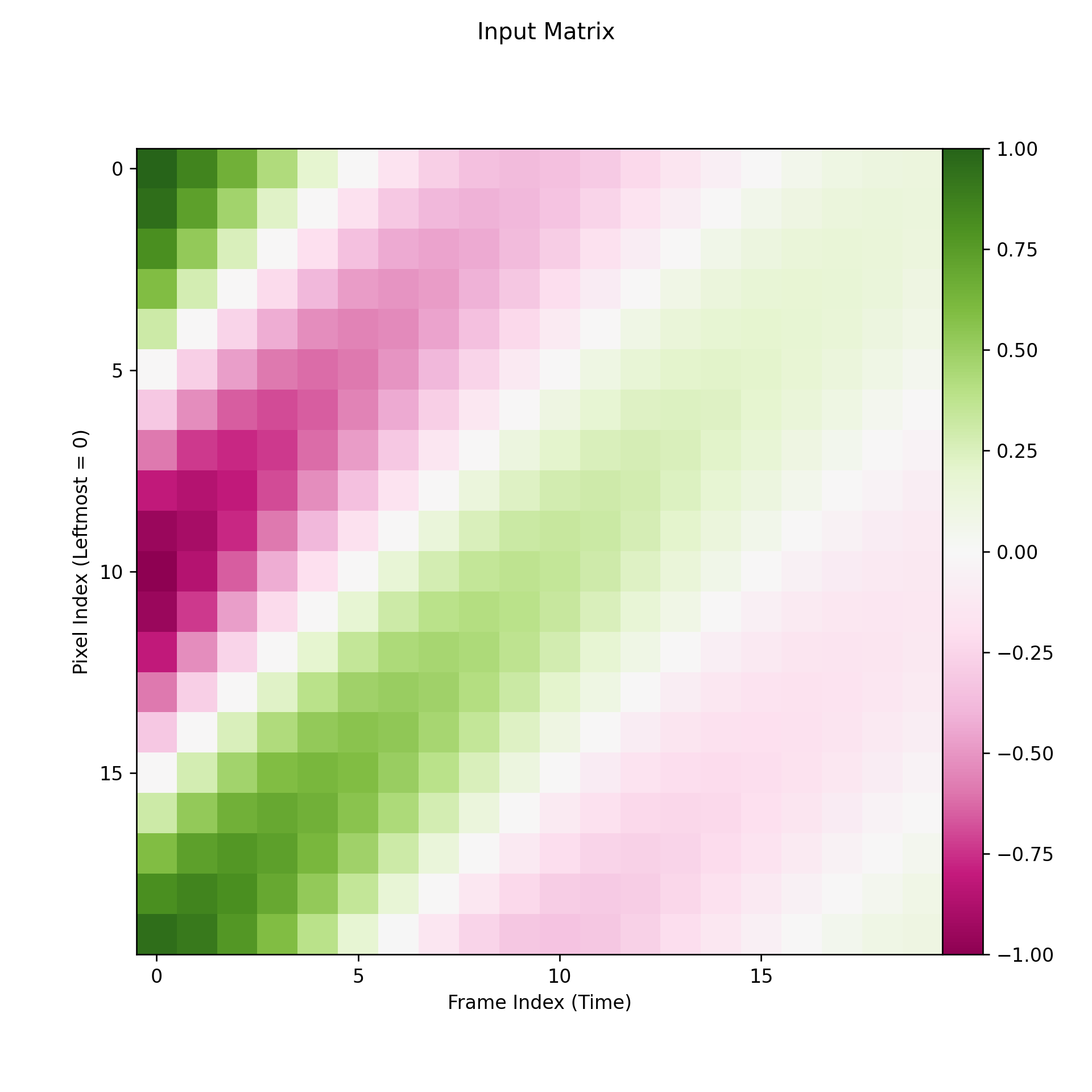
To start off, I’ve put together a toy example generated from a decaying, complex-conjugate pair of dynamic modes. This shows an ideal decomposition under the simplest possible circumstances.

Each pixel is an independent sample of a theoretical system we are decomposing, where dark green is the maximum positive value and dark purple the maximum negative value.

Set Up and Run the DMD

The first step is to organize our input into the matrix \(\mathbf{X}\), by joining all frames of the sequence as columns.

Input Matrix — The input matrix \( \mathbf{X} \). Each column is one frame of the previous video (rotated 90°), organized sequentially.

We now perform the dynamic mode decomposition on \(\mathbf{X}\), getting the dynamic modes \(\mathbf{\Phi}\), eigenvalues \(\mathbf{\lambda}\) and initial mode amplitudes \(\mathbf{b}\) (and from those, the initial mode amplitude diagonal matrix \(\mathbf{B}\) and dynamics \(\mathbf{C}\)).

Eigenvalues

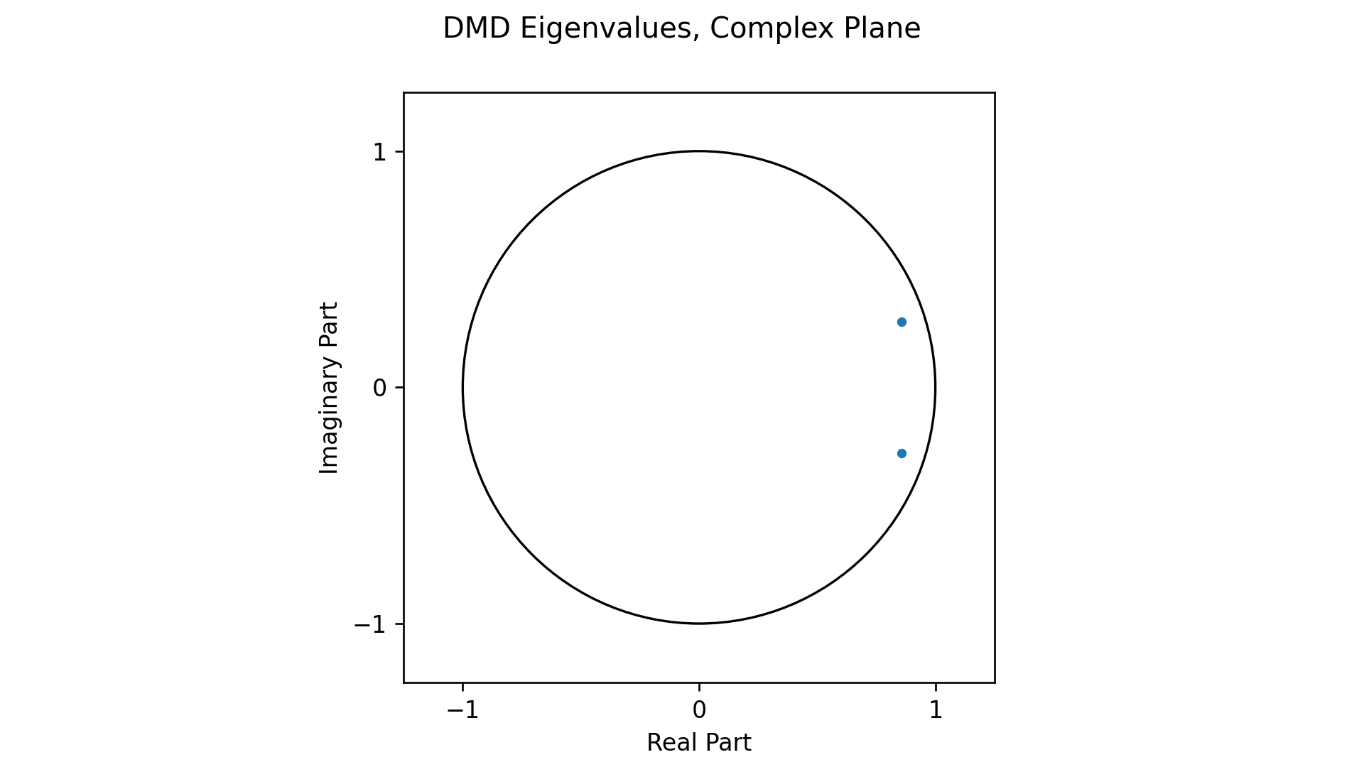
As expected, we see a single complex-conjugate pair of eigenvalues. By being inside the complex unit circle, their dynamics will decay over time. This is as expected and models the gradual fading seen in the input.

Reconstruction

We can see each DMD mode’s contribution to the reconstruction by multiplying each mode by its corresponding dynamic, individually:

\[\mathbf{X}_{DMD,i} = \mathbf{\Phi}_{*i} b_i \mathbf{C}_{i*}\]

Where \(\mathbf{\Phi}_{*i}\) is the ith dynamic mode (or column of \(\mathbf{\Phi}\)) and \(\mathbf{C}_{i*}\) the ith dynamic (or row of \(\mathbf{C}\)).

I’ve put both modes contributions, separated into real and imaginary parts, back into video form.

From top to bottom: the real contribution from the first mode, the imaginary contribution from the first mode, the real contribution from the second mode and the imaginary contribution from the second mode.

Notice how the imaginary components (second and fourth row) are equal in magnitude but of opposite sign (purple vs green). For real inputs, you should generally always get complex-conjugate pairs of eigenvalues that cancel out each other’s imaginary contributions. As such, the reconstructed output will also be real.

Ignoring these imaginary contributions which will cancel out, we can then visualize the contribution from each mode dynamic multiplication via a set of four matrices, one from the real parts of the inputs and one from the imaginary. The modes are represented by a color value, while the dynamics (premultiplied with their initial amplitudes) are shown as waves. I find this helps to highlight the spatial versus temporal nature of each.

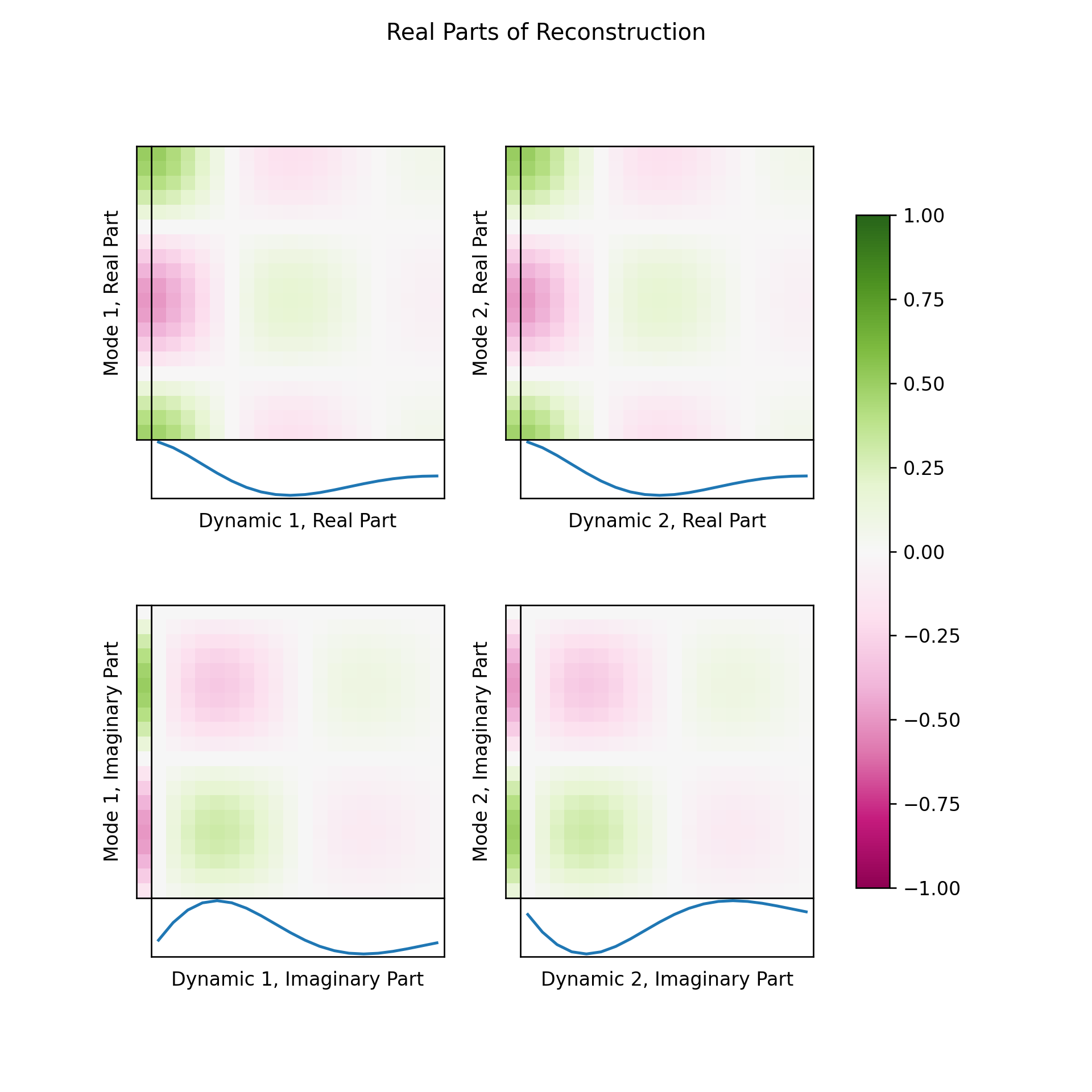
Reconstruction Components — The contributions made from each mode dynamic multiplication, separated by the real and imaginary parts of the inputs. Multiplications with imaginary outputs are not shown, as they cancel out to zero in the final sum. Note that the outer products in the bottom row are inverted because \( i * i = -1 \).

You can see in this figure how each half of this complex-conjugate pair of modes and dynamics is contributing the same thing to the output: a matrix equal to \(\mathbf{X} / 2\).

Background Subtraction

In my opinion, the coolest application of the DMD is to remove the background from video. Given a video with a fixed background, there will be a mode or modes with some \(\lambda \approx 1\). This represents a mode that is not only not growing nor decaying, but not oscillating at all.

I’ve made a synthetic example of a cube moving over a gradient to show how this works, as well as expected artifacting. Each frame of the input video is flattened into a single column of the input matrix \(\mathbf{X}\). By separating the mode with \(\lambda \approx 1\) from the rest and reconstructing, we can split out the foreground from the background as I’ve done in the following video:

A demonstration of using the DMD to split the foreground from the background.

Notice how the foreground is additive with the background, rather than containing the entirety of the foreground object. If we wanted to use this in practice for video segmentation, we’d want to do some kind of post-processing.

Plotting the eigenvalues on the complex unit circle and by \(\lvert \log{\lambda} \rvert\) helps to show what the background eigenvalue(s) looks like against the rest:

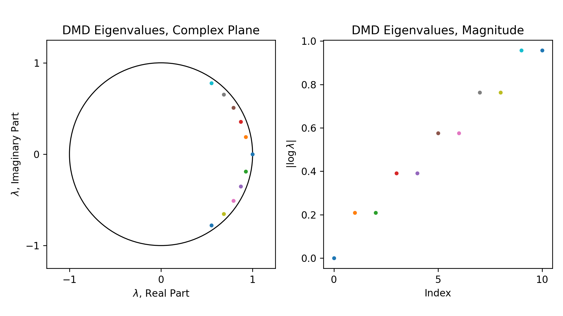
Background Subtraction Eigenvalues — On the left, the eigenvalues of the input video (above) plotted on the complex unit circle. On the right, these same eigenvalues sorted by their magnitude.

When the absolute value of the log of an eigenvalue is at or near zero, then it corresponds to the background, and vice versa. The eigenvalue corresponding to the background is that at the far right edge of the unit circle, on the left plot in the above figure, and at the origin on the right plot. In practice, one should threshold the split on a value near zero, and not exactly at zero.

Eigenvalues & Dynamics

In order to better understand the relationship between eigenvalues and dynamics, we can look at a simple example. I’ve plotted decaying (\(\lvert \lambda \rvert < 1\)), constant (\(\lvert \lambda \rvert = 1\)) and growing (\(\lvert \lambda \rvert > 1\)) eigenvalues, with varying phase angles, over 20 time steps on the figure below:

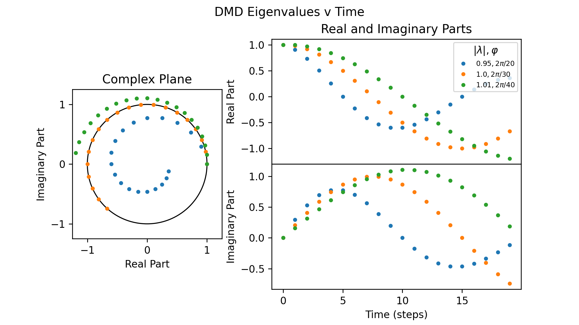
You can see how the further \(\lvert \lambda \rvert\) is from \(1\), the faster the dynamic’s amplitude grows or decays. Likewise, the greater the initial phase angle \(\varphi\) is, the further each step makes it around the complex unit circle and in turn the greater the frequency of the resulting dynamic. This is why the eigenvalues for the background of a video are \(\lambda \approx 1 + 0i\); this has a magnitude \(\lvert \lambda \rvert \approx 1\) and phase angle \(\varphi \approx 0\) which has little-to-no change over time.

This initial phase angle \(\varphi\) is calculated as follows:

\[\varphi = \arctan \frac{ \Im(\lambda) }{ \Re(\lambda) }\]

where \(\Im(\lambda)\) indicates the imaginary part of \(\lambda\) and \(\Re(\lambda)\) the real part.

Equivalently, we can reformulate \(\lambda\) to be calculated from the magnitude \(\lvert \lambda \rvert\) and initial phase angle \(\varphi\):

\[\lambda^t = |\lambda|^t (\cos \varphi t + i \sin \varphi t)\]

While understanding this relationship between eigenvalues and dynamics isn’t useful to using the DMD, I find it important to understanding how the DMD is representing the system.

Comparison With the Fast Fourier Transform

To show how the DMD is compares against the FFT practically, I’ve made another toy input designed to show a case that strongly favors the DMD. This is a sine wave of constant frequency that is decaying exponentially:

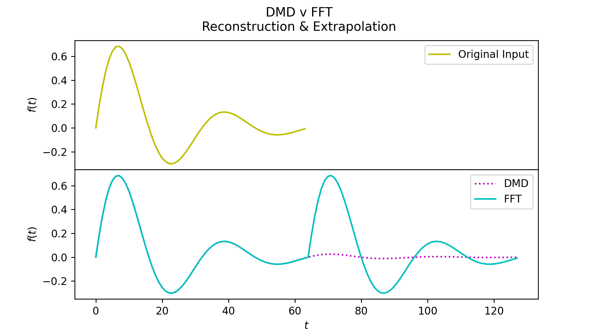
Signal and Reconstructions — Top: The input signal, which ends at \( t = 64 \). Bottom: Reconstruction of the input signal through \( t = 64 \), and extrapolation to \( t = 128 \) via both DMD and FFT.

While both algorithms can perfectly reconstruct the input, the extrapolation section highlights how the impact of the different ways they are representing the system. The Fourier transform assumes the system is periodic, and decomposes it into a set of fixed-frequency sine waves of constant amplitude. This means that extrapolating the FFT’s reconstruction into the future will continuously repeat the original input. As the DMD is instead modeling the system via sine waves with exponential growth or decay, the extrapolation will continue to grow boundlessly to infinity or shrink to 0.

If we plot the DMD eigenvalues and FFT frequency amplitudes next to one another, we can see how in this case the DMD more cleanly represents the system:

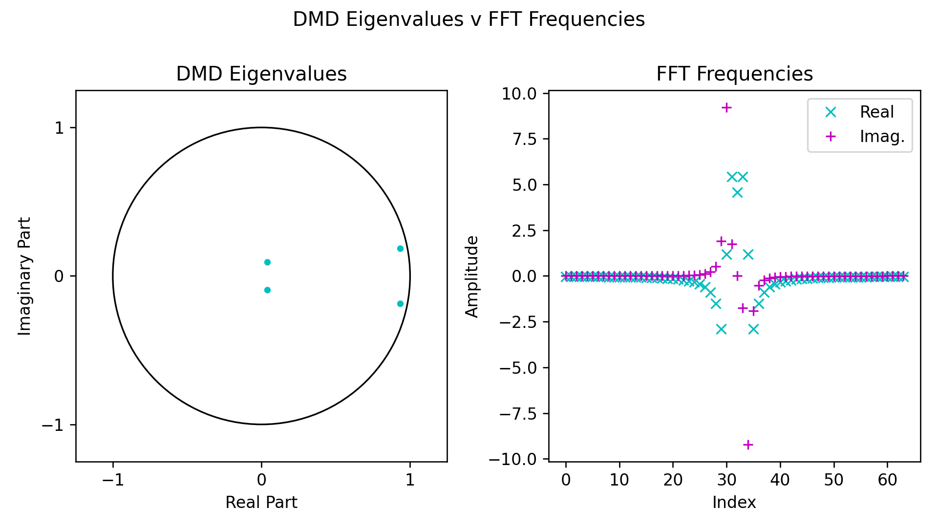
FFT v DMD — Left: The DMD eigenvalues generated for the above input. Right: The FFT frequencies generated for the above input. Notice that even if most of the low energy frequencies are removed from the FFT's output, it still represents the input via many more frequencies than that of the DMD (which needs two, via two complex-conjugate pairs).

Be aware that I specifically cherry-picked this example to show an obvious case where the DMD has a cleaner representation; this doesn’t mean the FFT isn’t useful here or elsewhere, just that the use of each algorithm has different repercussions.

As DMD eigenvalues encode frequencies, we can convert them into Hz with:

\[\mathbf{\omega} = \frac{ln(\mathbf{\lambda})}{\Delta t}\]

where \(\Delta t\) is the time difference in seconds between consecutive snapshots.

Algorithms

This section exists just so that I can quickly point people to an explanation of my college research project, the Streaming GPU Singular Value and Dynamic Mode Decompositions. I wouldn’t consider it to be particularly interesting otherwise, so no hard feelings if you stop here.

I will walk through how to calculate the SVD and DMD, and how to then use the DMD for background subtraction. Whenever there is a change for the Streaming versions, I’ve added a note with the details on what is different.

Note that below is just one possible way to calculate the Singular Value and Dynamic Mode Decompositions. I’ve chosen these versions because they are what we used for the Streaming SVD & DMD paper, but there are many other ways to calculate the SVD & DMD out there.

Dynamic Mode Decomposition

Find the Singular Value Decomposition (SVD) of \(\mathbf{X}_1\), the first through second-to-last columns of the matrix \(\mathbf{X}\) we are decomposing:
\[\mathbf{X}_1 \rightarrow \mathbf{U}, \mathbf{\Sigma}, \mathbf{V}^*\]
where \(\mathbf{U}\) and \(\mathbf{V}\) are the left and right singular vectors of \(\mathbf{X}_1\), and \(\mathbf{\Sigma}\) the singular values.
1. Find the eigendecomposition of \(\mathbf{X}_1^* \mathbf{X}\):
  \[\mathbf{X}_1^* \mathbf{X}_1 \mathbf{V} = \mathbf{V} \mathbf{\Lambda}\]
  This is a fast way to compute the SVD, taking advantage of the relationship between the SVD and eigendecomposition. This comes at the cost of a reduction in accuracy and limit to the number of singular values.
  
  🛈 Note
  Streaming SVD:
  As \( \mathbf{X}_1 \) will be updated at each frame by shifting all columns left by one, \( \mathbf{X}_1^* \mathbf{X}_1 \) will similarly be the same but with a shift up one row and left one column. We can take advantage of this fact, and only calculate that last row and column of \( \mathbf{X}_1^* \mathbf{X}_1 \) while just shifting the numbers in the existing matrix up and to the left. This significantly reduces the number of floating-point multiplications required on each update.
2. Calculate \(\mathbf{U}\):
  \[\mathbf{U} = \mathbf{X} \mathbf{V} \mathbf{\Sigma}^{-1}\]
  🛈 Note
  Streaming DMD:
  We don't need \( \mathbf{U} \) explicitly, so we can skip calculating it.
Form \(\mathbf{\tilde{A}}\):
\[\tilde{\mathbf{A}} = \mathbf{U}^* \mathbf{X}_2 \mathbf{V} \mathbf{\Sigma}^{-1}\]
where \(\mathbf{X}_2\) is the second through last columns of \(\mathbf{X}\).

🛈 Note
Streaming DMD:
We can insert the formula for \( \mathbf{U} \) from step 1.2 to make: \[ \tilde{\mathbf{A}} = (\mathbf{V} \mathbf{\Sigma}^{-1})^* \mathbf{X}_1^* \mathbf{X}_2 (\mathbf{V} \mathbf{\Sigma}^{-1}) \] This is much faster to calculate, and also lets us do something similar to step 1.1, by forming \( \mathbf{X}_1^* \mathbf{X}_2 \) from shifting \( \mathbf{X}_1^* \mathbf{X}_1 \) and only calculating the last column.
Perform an eigendecomposition of \(\tilde{\mathbf{A}}\):
\[\tilde{\mathbf{A}} \rightarrow \mathbf{W}, \mathbf{\Lambda}\]
where \(\mathbf{W}\) are the eigenvectors and \(\mathbf{\Lambda}\) the eigenvalues of \(\tilde{\mathbf{A}}\).
Create the matrix of dynamic modes \(\mathbf{\Phi}\):
\[\mathbf{\Phi} = \mathbf{X}_2 \mathbf{V} \mathbf{\Sigma}^{-1} \mathbf{W}\]
(Optional) Find the initial amplitudes \(\mathbf{b}\) of \(\mathbf{\Phi}\):
\[\mathbf{b} = \mathbf{\Phi}^\dagger \mathbf{x}_1\]
🛈 Note
Streaming DMD:
Instead, you can use the Fast Initial Mode Amplitudes (Fast b) formulation: \[ \mathbf{b} = (\mathbf{W} \mathbf{\Lambda})^{-1} (\mathbf{\Sigma} \mathbf{V}^*)_{*1} \] Where \( (\mathbf{\Sigma} \mathbf{V}^*)_{*1} \) is the first column of \( \mathbf{\Sigma} \mathbf{V}^* \). This is much faster to calculate, at the cost of a potential loss in accuracy.

At this point, we now have \(\mathbf{X} \rightarrow \mathbf{\Phi}, \mathbf{\Lambda} [, \mathbf{b} ]\). These are the dynamic modes, DMD eigenvalues and optional initial mode amplitudes, respectively.

Streaming Update Diagram — Streaming SVD and DMD work by taking advantage of the shared structure of \( \mathbf{X}_1^*\mathbf{X}_1 \) and \( \mathbf{X}_1^*\mathbf{X}_2 \).

Background Subtraction

To separate the background from the foreground, we continue from the above. If working with video, you will want each column of the input matrix \(\mathbf{X}\) to be a flattened frame; remember to unpack these afterwards before display.

Find which components don’t change over time, as follows:
\[\left| \log \lambda_i \right| \approx 0\]
Calculate the low-rank background matrix \(\mathbf{L}\):
\[\mathbf{L} = \sum_{i}\mathbf{\Phi}_i \mathbf{b}_i \mathbf{\lambda}_i^\mathbf{t}\]
Remove the background from the input matrix to create the sparse foreground matrix \(\mathbf{S}\):
\[\mathbf{S} = \mathbf{X} - \mathbf{L}\]
When working with real-valued input, you can discard the imaginary components of \(\mathbf{S}\) and \(\mathbf{L}\).

We are now done, and have \(\mathbf{X} \rightarrow \mathbf{L}, \mathbf{S}\), our final matrices containing the constant background and moving foreground, respectively.

Streaming DMD Engine Diagram — Diagram of how the Streaming DMD fits into a live background subtraction system.